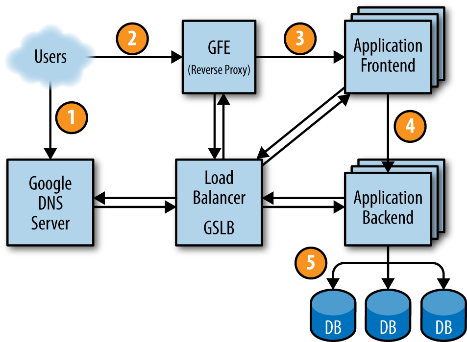
In the last blog post, we have introduced what a request may experiences when traveling from user’s browser to the data center. Now, the request finally reach the Application Frontend and front end is trying to communicate with back end.
Load Balance
Third Trial: RPC
In order to communicate with back end, front end can use REST way or RPC way. REST way is based on HTTP protocol; RPC way is based on TCP & UDP. Considering the efficiency of communication, google go the RPC way.
Along with RPC, they also adopted protocol buffer, which serialize data in binary which is faster and smaller than textual data which is used by HTTP protocol. In order to avoid the slow 3 way handshake when establishing connection and the slow start features, they make long-lived connection to backend servers. When a front end is quiet long enough, the TCP connection is closed to save cost and periodic UDP datagram is sent to do health check.
But in a data center, there may be exists more than hundreds or thousands of backend servers, it is impossible to hold connections to all backends. So we need to choose a subset of backends to connect. The first task is to choose a reasonable number for it. There exists no right answer for all system, it should be considered according to the number of front end and back end, traffic of data center, load of machine etc.
When the number is decided, we can use an algorithm to allocate the backends. The selection algorithm should assign backends uniformly but not fixed to handle machine failure and restart. A simple random selection method would fail because the variance is too large in practice:
def Subset(backends, client_id, subset_size):
  ratio =  subset_size / len(backends)
  return [i for i in backends if random.random() < ratio]
The algorithm provided by google is like following:
def Subset(backends, client_id, subset_size):
  subset_count = len(backends) / subset_size
  # Group clients into rounds; each round uses the same shuffled list:
  round = client_id / subset_count
  random.seed(round)
  random.shuffle(backends)
  # The subset id corresponding to the current client:
  subset_id = client_id % subset_count
  start = subset_id * subset_size
  return backends[start:start + subset_size]
Load Balance Algo
Now, we already kept the connection to some health backends, the next step is to send request with some strategy. The policy to do load balance can be very simple like Round Robin or a little bit complex, like Least-Loaded Round Robin, or combined with backends information Weighted Round Robin.
Round Robin
A simple round robin algorithm will send request to backends in set one by one, which is very simple, but has bad load balance result. The example in book showed that this may result in 2 times gap in CPU load from the least to the most loaded backends. It may comes from the following reason:
- Too mall subsets and different loaded client;
- Unbalanced cost to handle different requests;
- Differences between machine;
Least Loaded Round Robin
This algo require the client to remember the number of active requests it has to each backends, and use Round Robin among the set of tasks with minimal number of active requests. In practice, they found the service using Least-Loaded Round Robin "will see their most loaded backend using twice as much CPU as the least loaded, performing about as poorly as Round Robin.
Weighted Round Robin
The core reason that the above algorithm fail to do a good job on load balance is the client don’t know the state of backends (or choose a bad criterial to estimate as Least Loaded Round Robin does).
The Weighted algo make load balance decision based on the info provided by backends. It will keep a score for backends and update the score according to the response backends give. Backends will include the rate of queries and errors per second, in addition to the system load – usually, CPU usage. And this algorithm indeed get very good results in production as book introduced.
Finally, the request reach the backends, the next step to DB is relatively similar with previous step, as now Backends is the client and DB is “back end”, so the techniques also works. And this is the end of story.
Written with StackEdit.

评论
发表评论